Bound to extremes

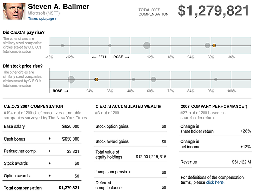
The New York Times continued to push the envelope by printing super-complicated data graphics (while the Economist regrettably seemed to have picked the USA Today route... more on that in a future post).  The following graphic was used to illustrate the relationship between CEO compensation and their company's stock performance.

The two dotplot lookalikes depicted the percent change in CEO pay and the change in companies stock price, in both cases, from 2006 to 2007.  The size of the dots indicates the relative value of the CEO's pay.  The gray dots depict "similarly sized" companies for comparability.

In this post, I will focus on the comparison between change in pay and change in stock price for a given CEO.  In particular, the calibration of the axis/scale is problematic.  The scale is automatically determined by an algorithm; as one switches from one CEO to another,  the graphs take on different ranges, use different axis labels, and the zero-percent points shift.

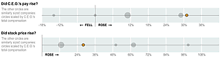
This means that the two charts have different scales.  In this example, each tick mark advances 6% in the top chart but 12% in the bottom chart.

Since the zero points do not line up, the distance between the zero and the orange dot loses meaning:  the 2.5x longer distance in the top chart actually represented the same percentage change as in the bottom chart (31% versus 28%).

In order to respect the grid-lines (white lines), the tick marks fall onto stray percentages (24%, 36%, 48%, etc.).  That's unfortunate.

What's the culprit?  This chart is "bound to extremes".  In other words, the range of the depicted data is used to determine the plot area.  The bottom chart had zero on the left edge because all the stocks depicted rose between 2006 and 2007.  It is often better to use domain knowledge to determine the plot area.  Extreme values should be omitted if they don't add to the message.  Oftentimes, by leaving extreme values in the picture, we squash the rest of the data.

This is also why programs like Excel do a poor job picking a scale.

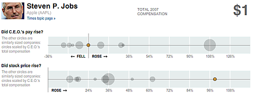
As an aside, the use of bubbles is almost always troubling. Bubbles do not have a scale so the only information we get is relative size.  However, we can't estimate areas properly so we get the relative size wrong.  Sometimes, even the chart designer may get stumped.  In the chart of Steve Jobs, you would think his bubble (total compensation $1) would be dwarfed by all the other bubbles, as in the WSJ chart we showed the other day.  Not so.

Thanks to Todd B. for submitting this chart.

Reference: "Executive Pay: the bottom line for the those at the top", New York Times, April 5 2008.