Primer on Regression Adjustments 1

I was once asked to write five learning objectives for some 30 lectures of a semester-long course -- amounting to over 100 bullet points possibly read fewer than 100 times in total by the students. My syllabus was summarily rejected; it probably caused a five-alarm fire in some dean's office. For example, the learning objective submitted as "Understand when to use regression analysis, and how to interpret the results" displeased because this outcome is not "measurable". I didn't argue with that and dutifully changed it to "Execute the five steps of running regression analysis", which read like gold to the currriculum board.

This is a nugget of what's wrong with statistics education. Our students can mechanically write code to run all kinds of models but they don't learn how to think critically about what they have just produced. In a series of posts, starting today, I present some materials on regression analysis that you won't find in a standard statistics textbook. At the end of this series, I hope you come away realizing that regression is a useful tool but it is not a magic wand that fixes all problems.

A lot of recent scholarly papers on the pandemic uses regression to "correct for" biases in the real-world datasets. Observers are hoodwinked into thinking that regression cures all biases. For example, even John Burn-Murdoch at the Financial Times tweeted the following a few days ago, citing a number of experts he talked to:

John believed that regression effectively cured "a huge list of confounders". You won't believe that after you finish this series of posts about regression adjustments.

***

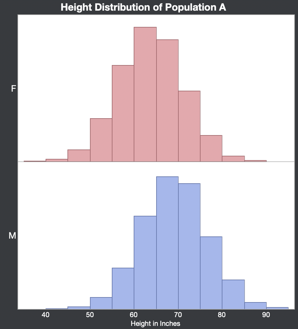
We start with a Population A of 25,000, split evenly male and female. We have data on their heights in inches. (1 inch = 2.5 cm, 1 feet = 12 inches = 0.3 m, 1 metre = 3.3 feet = 39 inches).

The following tabulation confirms the gender ratio. The population average height is 66.5 inches (5.5 feet).

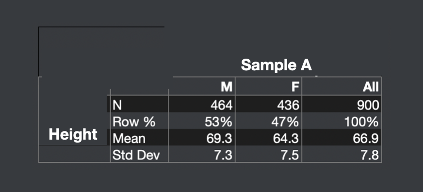
An analyst is given Sample A, which contains 900 records taken from Population A. These records are randomly selected from the population. The average height of the 900 people ("sample average") is 66.9, which is tantalizing close to 66.5. As you learned in Stat 101, this is the beautiful foundation of statistics. You can take the sample average, and use it to estimate the population average height, and you'd be very close.

How close? This is measured by the "standard error", which is 7.8/sqrt(900) = 7.8/30 = 0.26 inches. The standard error is the building block of the familiar concept of "margin of error", which is +/- 2 standard errors. Thus, the margin of error in this case is ~0.5 inch on either side of 66.9. The range is 66.4 to 67.4. Statistical theory predicts that 95% of the time, the true average height in the population is found in this range, and indeed, our sample is part of this 95%.

For later reference, just remember that 0.5 inch (12 mm) is a big error on this scale. Half an inch is the difference between the median person sample and the 97.5th percentile person sample. So our tolerance for inaccuracy is described in small fractions of an inch.

We now exit this perfect world, in which the sample of data received is a random sample of the population, that is to say, contains no biases. Almost all real-world datasets are going to suffer from selection biases.

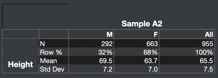
The analyst receives a new dataset, Sample A2, also of 900 people, and determines the sample average height to be 65.5 inches. Inspecting the gender of Sample A2, the analyst discovers that it contains 70% females and 30% males.

Since females on average are shorter than males, the sample average height of 65.5 is below the population average height of 66.5. The difference of 1 inch is a major error, as we learned from the calculation above.

Sample A2 has a selection bias favoring women. The analyst now waves her magic wand. It's called "regression." She is now going to "adjust" or "correct" the sample estimate for gender bias. The gender-adjusted sample average height is 66.6 inches. This number comes from the constant term of the following regression model:

66.6 + 2.9 if Male - 2.9 if Female

The adjusted number of 66.6 is almost exactly the average height of the population of 25,000. Thus, regression has magically removed the gender bias and delivered an accurate estimate of the population average height. What's not to like?

This is where most textbooks end the discussion. Quod erat demonstrandum.

For me, this is where the class starts.

***

Before the next post, I leave you with the following questions to ponder:

In the real world, we don't have access to the population dataset. We don't know what the population average height is, nor do we know what the gender ratio is in the population of 25,000. All we have is the sample of 900 people. Does the software executing that regression know that the sample is biased?

If you think the software knows, then how does it know?

If you think the software doesn't know, then what is it correcting?

P.S. [8-27-2021] Post 2 is now up. It contains the answer to the above question.

P.S. [9-1-2021] Post 3 explains why "removing" the effect of gender ironically acknowledges its importance.